I recently got an email saying:
I realised that no, there is no such tutorial and had the idea to dedicate a discussion thread to this topic.
So lets start.
QUOTE:
I installed a trial version of Finantic.Optimizers for Wealth Lab 8. Do you have any tutorial showing the features and how to use the extension within WL8.
I realised that no, there is no such tutorial and had the idea to dedicate a discussion thread to this topic.
So lets start.
Rename
What is an optimizer?
What happens if you develop a trading strategy?
You build some logic (ether building blocks od´r C#code) for a trading strategy until it produces some results in a backtest.
Then you start to vary the logic, used indicators parameters and so forth.
Each time some after some change is implemented you check the results to see if the strategy "improved". I.e if the perforamnce metrics you consider most important get better.
This is a time consuming, boring and error prone process.
Within WL8 thre is a piece of software which can help in varying the parameters of your strategy and observe the results (a set of performance metrics).
The software that can do this automatically is called an "Optimizer".
It works as follows:
The Optimzer looks at your strategy and finds all "optimizable paramters" with their respective min-values and max-values. Then it runs your strategy with sveral combinatoons of parameter values and records the result with the goal to find a paramter combination that works better than the rest.
This is the basic inner working of every optimizer algorithm. They differ in some details, which is described in the next post.
The Builtin Optimizers
WL8 comes with two optimizer algorithms: Exhaustive and Shrinking Wndow.
Exhaustive Optimization
When you specify an optimizable paramter for your strategy, you specify:
* Default Value
* Min Value
* Max Value
* Step size
The exhaistive optimizer will use parameter values between Min-Value and Ma-Value that lie "Step Size" apart.
Example:
If you use an ATR indicator, this indicator has an "period" paramter.
If you make this paramter optimizable you may specify:
* Min-Value=2
* Max-Value=12
* Step Size = 2
With this information the exhaustive optimzer will use these values for the ATR period:
2, 4, 6, 8, 10, 12
It starts with Min-Value, adds the Step-Size again and again unitil the Max-Value is reached. In this case the strategy is run 6 times.
If there are two optiizable paramters the exhaustive optimizer will use all possible values for both parameters. If a second parameter has 3 different value this will result in 6 * 3 = 18 runs of the strategy.
With more paramters the number of necessary runs will grow very high. I.e an optimization run with exhaustive optimizer can easily take a long time.
On the other hand: With exhaustive optimizer you can be sure that you get results for every possible combination of paramter values.
Shrinking Window
The shrinking window optimizer is a bit more clever than the exhaustive optimizer.
It starts with wider steps through the parameter space and zeros-in when it finds some promising paramter combinations.
That way it needs fewer runs to find a good combination than exhaustive.
On the other hand there is always the risk to miss the "true best parameter combination"
In most cases "Shrinking Window" is more useful that "Ehaustive" simply because it is much faster.
The finantic.Optimizers algorithms
The finantic.Optimizers extension comes with a set of additional optimizer algorithms.
Most of them have their merits in some situations, so let me describe what these algorithms do and what are their applications.
Nelder Mead
The Nelder-Mead algorithm (https://en.wikipedia.org/wiki/Nelder%E2%80%93Mead_method) is mainly interesting for historical reasons. It was one of the first widely known algorithms which worked in multi-dimensional spaces. Unfortunatel this algorithm makes some assumptions about the "landscape" which are seldom met by trading strategies. So in most cases it works poorly for trading system development.
Bayesian Optimization
This one is more modern than Nelder Mead but also makes some assumptions about the paramter space which usually don't hold for trading strategies. It is a bit better than Nelder Mead but not as good as the other available algorithms.
Particle Swarm
This algorithm combines two interesting ideas:
First, there run several searches in parallel, each search being a "particle". This improves the chances to find a good solution.
Second: It copies a basic principle of evolution: Only the best survive.
Both ideas combined result in a powerful algorithm, which is fast and finds good solutions.
Before I write about the "best" algorithm, let me explain two special purpose optimizer algorithms.
Grid Search
The Grid Search algorithm works similar as the Exhaustive algorithm. There are two important differences however:
First, with Grid Search you specify the number of iterations you are willing to wait for.
The algorithm than works backwards and finds step-sizes for each parameter which will result in (roughly) the number of iterations requested.
Second, Grid Search does not respect the step-size specified in your optimizable parameter declarations. Insteads it chooses a step-size which allows for the requested number of iterations.
This results in these properties for the Grid-Search algorithm:
* Limited run time because you can choose the number of iterations
* The complete parameter sapce is searched (Like Exhaustive)
This algorithm is a good choice if you are interested in a "first overview" of your parameter space.
I use this algorithm for a new/unknown strategy with one or two optimizable parameters to get an impression where the "working" paramter values are and what results are to expect.
If these results look promising I start to restrict my parameter space, I choose more tight values for Min-Value and Max-Value of each parameter.
Then I use one of the more powerful algorithms to find better results with higher precission.
Random Serach
As the name implies this algorithm chooses parameter values randomly (between the defined Min-Value and Max-Value boundaries of every paramter)
This is a very powerful method if you have no clue what you are dealing with.
I.e if there is a new or unkown trading strategy with many paramters then the Random Search is one of the best methods to find "workable" parameter sets and a rough impression about possible results.
If such results are promising I make the search-space smaller by restricting Min-Value and Max-Value of all the parameters. This can be done by observing the "Parameters and Metrics" Optimization Results Visualizer. (This one is explained in another post)
With the smaller paramter space I then continue with one of the more powerful optimizers.
SMAC
This is my fafourite optimizer algorithm. It can handle a large number of optimizable paramters and still find very good parameter combinations with a rather small number of iterations.
The SMAC optimizer is that good because it combines the best features of several other optimizer algorithms:
* Random Search
* Particle Swarm
* Hill Climbing (without any assumptions about the "landscape")
BUT: You need reasonable parameter boundaries (Min-Value and Max-Value) to start with. Otherwise the random startup sequence of SMAC will not find enough valid results to start any reasonable optimization.
With a new or unknown strategy you should start with Grid Search or Random Search to find reasonable boundaries for your parameters.
Once this is done you should continue with SMAC to find very good results with a low number of iterations, for example 500 or 1000 runs.
A comparison of the various optimizer algorithm can be found in ths thread:
https://wealth-lab.com/Discussion/Choosing-the-best-Strategy-optimizer-6707
It clearly shows how the SMAC optimizer is much better than all the other algorithms.
https://wealth-lab.com/Discussion/Choosing-the-best-Strategy-optimizer-6707
It clearly shows how the SMAC optimizer is much better than all the other algorithms.
This great article belongs to the Blog section: https://www.wealth-lab.com/Blog
Good idea.
DrKoch, would you mind submitting this as a blog in a markdown format with any supporting images? Or we could copy it and format it too. It's more visibility for you extension(s).
DrKoch, would you mind submitting this as a blog in a markdown format with any supporting images? Or we could copy it and format it too. It's more visibility for you extension(s).
QUOTE:
Or we could copy it and format it too.
This thread is work in progress. I plan to add more information here.
Please let's wait until it looks finished.
QUOTE:
would you mind submitting this as a blog in a markdown format with any supporting images?
I feel like the blog format is too rigid for me. I can't submit a complete article from start to end in one go. Rather I need some format with remarks, questions, suggestions, some text added later, edits, improvements and so forth.
The discussion group format comes close but is not ideal. The best would be some wiki format where I (and everybody else) can improve/optimize the text (and images) over time.
For sure we can wait with publishing to the blog until your important work is finished - and post timely updates later when required - if the post contents are Markdown formatted.
Making their way through multiple posts may be inconvenient for the readers, but cross-linking the blog post to this thread for a community discussion is an affordable alternative to another entity like wiki (which is a security concern as these engines get hacked more often than other).
Making their way through multiple posts may be inconvenient for the readers, but cross-linking the blog post to this thread for a community discussion is an affordable alternative to another entity like wiki (which is a security concern as these engines get hacked more often than other).
Back to the optimizers.
With such many algorithms available it can be overwhelming to find the right choice for the task at hand so let me add some more information.
Requested Number of Iterations
There are two types of optimizer algorithms. With he first group the number of iterations is calculated indirectly. It results from parameter properties like Min-Value, Max-Value and Step-Size for the Exhaustive Optimizer. It is the product of Outer Passes and Inner Passes for the Shrinking Window algorithm.
On the other hand there all the other algorithms form the finantic.Optimizers extension. With these algorithms it is possible to specify the (approximate) number of iterations directly. This is often more convenient.
Required Number of Iterations
One important goal in trading system development is to find a very good strategy as fast as possible. You don't want to waste time waiting for a long running optimizer session if there are ways to achieve the same results in much less time.
The algorithm comparison mentioned in Post #9 shows that the various algorithms can make a huge difference if it comes to the number of required iterations to reach a good result.
Dump Algorithms vs. Smart Algorithms
This somewhat provocative section heading is misleading. In fact there are no dump algorithms.
A better title would be Guided vs. Unguided algorithms.
An unguided algorithms simply chooses a set of parameter combinations without taking any results into account.
The big advantage of such an algorithm: It works always, no matter what the trading strategy is doing.
Even if there are no results for many paramter sets it will show you exactly that result: No results for many parameter combinations.
It is adviceable to use such an algorithm if not much is known about a strategy and their useful parameter ranges.
Unguided algorithms are:
* Exhaustive (low number of optimizable parameters)
* Grid Search (low number of optimizable parameters)
* Random Search (higher number of optimizable parameters)
A Guided algorithm observes the results of some initial parameter combinations and chooses new parameter sets
taking these results into account. This allows for ideas like "Hill Climbing".
A guided algorithm has a setting "Target Metric" and it tries to maximize this metric while it runs.
The advantage of such an algorithm: It concentrates on "interesting" regions and does not waste CPU cycles calculating results that will never be used again.
On the other hand such a guided algorithm needs enough valid results from initial or previous runs.
If the allowed parameter ranges result in too many runs without any result, such an algorithm will fail. This means that you should already know what parameter ranges are useful.
Guided Algorithms are:
* Bayesian
* Nelder Mead (The mother of all guided algorithms, not very useful for trading strategies)
* Particle Swarm
* Shrinking Window (fast)
* SMAC (very fast)
Summary I: How to choose an optimizer algorithm
If I am to choose one of the optimizer algorithms I proceed as follows:
As long as I have a new or unknown strategy I want to learn how different parameter values influence the outcome of that strategy.
If I am interested in a single parameter I use Exhaustive or Grid Search with a broad parameter range.
Sometimes I have two optimzable parameters which are somehow related. In this case I use Exhaustive because it can produce a nice "Mountain".
(More about results of optimizer runs in a later post)
If there are more than two parameters and as long as I don't know much about the strategy I use Random Search to find parameter ranges that produce meaningful results.
With all these results in mind I start to restrict the parameter ranges.
(Here the Parametrs and Metrics Visualizer is helpful, again: more about this in a later post)
I try to find Min-Values and Max-Values for each parameter that make sure that some results are produced without restricting the search space too much.
Now it is time for the SMAC optimizer which can handle a larger number of parameters and finds very good results with a relatively small number of iterations (say 500).
Target Metric?
A guided algorithm has a setting "Target Metric" and it tries to maximize this metric while it runs.
Fine. But which one should I choose?
This question is ralated to "Which is the best performance metric?"
A question which is not easy to answer.
Lets observe what a human system developer is looking at:
First: Profit. Of course we are interested in earning some money.
We'll used the annualized profit as a percentage (APR) to make the numbers comparable between various backtests.
This one was easy. Or not?
APR depends on position size which is easily changed. A more stable metric is average profit per trade in percent,
but this one is more abstract and does not show you the $$$ directly.
Next: Risk. No profit comes without risk and it is important to quantify/measure this risk also.
All practitioners are interested to know the Drawdown. Maximum Drawdown (MaxDD).
Unfortunatly this metric depends on a lot of things:
* Position size (see above)
* Data Range. (Yes, often forgotten: The larger your data range, the larger Max Drawdown (on average))
* Worst: Max.Drawdown depends (only) on a handful of trades, so it will never repeat itself and it is rather unstable. If you change your portfolio somewhat the MaxDD can change a lot.
There exists a nice solution called "Expected Drawdown". It uses some fancy math (called the bootstrap) to calculate a probable number of DrawDown.
This one is much more robust against changes in the Portfolio. It comes with the finantic.SysQ extension (which is free).
Better: A Risk/Reward Ratio. These usually do not depend (much) on position size and so forth.
The etablished gold standard is Sharpe Ratio based on monthly equity changes.
I prefer the Sharpe Ratio based on daily equity changes. (Comes with the finantic.ScoreCards extension)
There are many more risk reward ratios, all highly correlated, so it does not make much of a difference which one you choose.
Also important: Number of positions: Is this a practical strategy or has it theoretical value only? (too few or way too much trades?)
With WL and limit order systems we want to keep an eye on NSF ratio.
And everyone has some more metrics they like to observe.
So again:
Which one is best suited as a Target Metric for a guided optimizer algorithm?
From the discussion above it seems most preferable to use one of the risk/reward ratios.
If you do this you'll discover something strange: The optimizer algorithm will (of course) find a parameter combination which results in the best possible risk/reward ratio.
This often results in a strategy which enters just one or two winning trades. Very good risk/reward ratio but very low profit. And completely not practical.
So these risk/reward ratios are usually not a good fit for Target Metric of a guided optimization algorithm.
The solution seems to be some combined Performance Metric. The resulting method is called Multi-Objective Optimization.
(see https://en.wikipedia.org/wiki/Multi-objective_optimization)
It can be done with the FormulaScoreCard (part of the finantic.ScoreCards extension). It is a field of research and deserves its own discussion thread.
Until I find some good Combined Performance Metric I stick with APR for Target Metric and closely observe the other metrics mentioned above for the best candidate strategies found by the optimizer.

Thank you very much for sharing this!
I have the relevant Finantic extensions since they were launched, but this info certainly helps to extract more value from them.
I have the relevant Finantic extensions since they were launched, but this info certainly helps to extract more value from them.
QUOTE:
this info certainly helps to extract more value
Thanks for the encouraging words.
Getting Started
Now that we have a reliable map with available algorithms, various pathways and possibilities it is time to get our feet wet and find our own ways.
What follows is a step by step tutorial about optimizing and making the most of an existing strategy.
I'll assume a reader who conducted some backtests with Wealth-Lab but never run an optimization.
So lets get started...
Phases of Trading Strategy Development
... before we start it is important to recognize that there are various phases the development of a trading strategy goes through. We have to make quite some decisions along the way and the proper decision depends on the phase we are in, so it is good to know.
The sequence of phases is:
Exploration
This is all about the strategy's trading logic. Is the logic able to produce profitable trades? What is the character of the strategy? How does it react to parameter changes? In this phase we completely ignore practical considerations like the money in our account or the restrictions of the broker or the rest of real life. We concentrate on the trade logic, its possibilities and its boundaries.
Fine Tuning
In this phase we have a narrow range for each parameter. We are concerned with stability and robustness.
Adding Realism
Now we take our exiting broker account into account. How much capital is available for this strategy? Which position sizes? How many trades are possible? Margin? Is the strategy even tradeable with the effort we are willing to put in?
Validation Backtest
With all settings and adjustments fixed we run a single validation backtest on unseen data. If the results are not good enough the strategy does not survive this phase. We'll throw it away and start all over with phase 1.
Paper Trading
At this stage we are confident that we found a working profitable trading strategy. We conduct a certain phase of paper trading with a simulation account. And compare the results to backtest results. The details of this phase are beyond this text.
Realtime Trading
After paper trading was successful we start real trading with real money. This phase is beyond this text also.
Step 0: Find a Trading Strategy
Before we are able to optimize a strategy we need one. There are many ways to find a strategy to start with:
Internet (YouTube and friends)
There are many. The probability to find something that survives a backtest in WL is low.
Books and Journals
Same as above. With one notable exception: Laurens Bensdorp published a book with strategy that seem to work.
(see https://www.wealth-lab.com/Discussion/Laurens-Bensdorp-s-Automated-Stock-Trading-Systems-9377)
Strategy Genetic Evolver
This is an exciting tool within Wealth-Lab which can produce new trading ideas. Very promising. The strategies found by this evolver a perfect candidates for further optimization.
Published Strategies
see https://www.wealth-lab.com/Strategy/PublishedStrategies
These are great candidates with the big advantage that these strategies are already available for WL backtests, ready for optimization.
Top 5 Published Strategies
The most promising candidates.
For this tutorial we'll select one of the strategies of the Top 5: OneNight.
This is the simplest profitable strategy I can think of.
Step 1a: Make a Building Block Strategy Optimizable
We start with a building block version of the OnNight strategy:

It is just one Entry Rule: Buy at Limit 2% below Close
and one Exit Rule: Sell at Market.
If we look cursorily we discover just one thing to optimize, it is the "2%".
In fact we find us in the Exploratory Phase (see above) and ask the question: What happens if I change this number?
So we want the optimizer to change this number for us, we want to make this number optimizable.
To do so we find the gearwheel button (see red rectangle in the screen shot above)
If we click this button we can modify the settings for the entry building block:
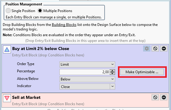
Next to the Percentage setting there is a button "Make Optimizable.." (see red rectangle). If we click this one it opens another Dialog "Parameter Optimization Settings":
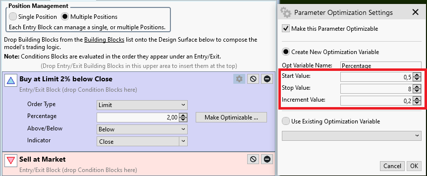
This dialog allows us to set:
* Start Value
* Stop value
* Increment Value
for the parameter "Percentage". We'll talk about good choices in one of the next posts.
If we close this dialog and save the strategy we're finished. We did change the OneNight Strategy into an optimizable strategy. Congrats!
We start with a building block version of the OnNight strategy:
It is just one Entry Rule: Buy at Limit 2% below Close
and one Exit Rule: Sell at Market.
If we look cursorily we discover just one thing to optimize, it is the "2%".
In fact we find us in the Exploratory Phase (see above) and ask the question: What happens if I change this number?
So we want the optimizer to change this number for us, we want to make this number optimizable.
To do so we find the gearwheel button (see red rectangle in the screen shot above)
If we click this button we can modify the settings for the entry building block:
Next to the Percentage setting there is a button "Make Optimizable.." (see red rectangle). If we click this one it opens another Dialog "Parameter Optimization Settings":
This dialog allows us to set:
* Start Value
* Stop value
* Increment Value
for the parameter "Percentage". We'll talk about good choices in one of the next posts.
If we close this dialog and save the strategy we're finished. We did change the OneNight Strategy into an optimizable strategy. Congrats!
Step 1b: Making a C# Coded Strategy Optimizable
As an example we use the OneNight strategy, this time the C# Coded variant. It looks like this:
If we look cursorily we discover one parameter. It is the "percentage," which is set to 2.0 %.
To make this strategy optimizable we introduce a parameter with a call to AddParameter(). This is done in the strategy's constructor, because it is done just once:
This call accepts:
* a good name for the parameter
* the type of this parameter, can be integer or double
* a default value
* a start value
* a stop value
* an increment value
We'll talk about a good choice for Start, Stop and Increment in another post.
With this call in place we can replace the constant "2.0" by our newly created parameter:
That is it! With these two code changes we created an optimizable C# coded strategy.
Here is the complete code:
As an example we use the OneNight strategy, this time the C# Coded variant. It looks like this:
CODE:
using WealthLab.Backtest;
using WealthLab.Core;

namespace WealthScript10
{
    public class MyStrategy : UserStrategyBase
    {
        public override void Execute(BarHistory bars, int idx)
      {
         double percentage = 2.0;
         foreach (var pos in OpenPositions) ClosePosition(pos, OrderType.Market);
         double limit = bars.Close[idx] * (1.0 - percentage / 100.0);
         PlaceTrade(bars, TransactionType.Buy, OrderType.Limit, limit);
        }
    }
}
If we look cursorily we discover one parameter. It is the "percentage," which is set to 2.0 %.
To make this strategy optimizable we introduce a parameter with a call to AddParameter(). This is done in the strategy's constructor, because it is done just once:
CODE:

public MyStrategy() : base()
{
      AddParameter("Percentage", ParameterType.Double, 2, 0.5, 8, 0.2);
}
This call accepts:
* a good name for the parameter
* the type of this parameter, can be integer or double
* a default value
* a start value
* a stop value
* an increment value
We'll talk about a good choice for Start, Stop and Increment in another post.
With this call in place we can replace the constant "2.0" by our newly created parameter:
CODE:
double percentage = Parameters[0].AsDouble;
That is it! With these two code changes we created an optimizable C# coded strategy.
Here is the complete code:
CODE:
using WealthLab.Backtest;
using WealthLab.Core;

namespace WealthScript10
{
    public class MyStrategy : UserStrategyBase
    {
      public MyStrategy() : base()
      {
         AddParameter("Percentage", ParameterType.Double, 2, 0.5, 8, 0.2);
      }

        public override void Execute(BarHistory bars, int idx)
      {
         double percentage = Parameters[0].AsDouble;
         foreach (var pos in OpenPositions) ClosePosition(pos, OrderType.Market);
         double limit = bars.Close[idx] * (1.0 - percentage / 100.0);
         PlaceTrade(bars, TransactionType.Buy, OrderType.Limit, limit);
        }
    }
}
.. but if you're optimizing a parameter used by an indicator - usually instantiated in Initialize() - there's one more step to make the strategy compatible with WFO (Walk-Forward Optimization). Dr Koch will probably mention that next :)
QUOTE:
WFO (Walk-Forward Optimization). Dr Koch will probably mention that next
Well WFO is for later, much later...
Choosing Start, Stop and Increment Values for Optimizable Parameters
It turns out that this seemingly small detail is a rather important and sometimes critical one.
If the parameter range is too wide, i.e. Start too low, Stop too high then you are going to waste CPU cycles and lifetime while waiting for the optimizer to finish while it will return a lot of useless results. And some optimizer algorithms (like SMAC) may even fail if the parameter ranges are too wide and too many parameter settings don't produce trades or otherwise invalid results.
On the other hand, if the range is too narrow, i.e. start too high , stop too low then you don't "see" the interesting part of your parameter space. You'll miss the true best parameter value.
Similar with Increment value: If this is too small, the optimizer will take too much time and CPU power to step through narrow spaced values without adding enough information to the results.
If it is too large the result could be too coarse, again hiding the true best parameter value. Luckily the Increment value is of concern for just a limited set of optimization algorithms (namely Exhaustive and Shrinking Window), all other algorithms will ignore the Increment and choose their own step sizes while varying the parameter values.
All of this discussion gets even more critical if there are several parameters.
Don't panic, as we will see later we can use the results of one optimization run to improve on the parameter ranges for the next one. It is just important that we do improve the parameter ranges over time.
Practical Tips
Ok, before you get lost in dos and don'ts here some practical tips:
In the example above we started with a working strategy, i.e. a strategy that had some parameter values which produced some useful results.
When I turn such a strategy into an optimizable one, I replace the interesting numbers by an optimizable parameter. While in Exploration Mode (see Post #23 above) I tend to choose a Start Value 2-4 times slower than the original value.
(Here we had 2% for original, so Start is 0.5% to give a good overview)
Accordingly I choose the stop value 2-4 times higher than the original (here 8%).
When I plan to use the Exhaustive Optimizer I go for 20 to 100 Iterations, in the example above I arrive at an Increment 0f 0.2% which will result in (8-0.5)/0.2 = 37 Iterations.
Later, In Fine-Tuning Mode I try to get parameter ranges where the Stop Value is 1.5 to 3 times higher than the Start Value. We'll see this later.
We're getting closer. But before we can produce our first optimization results we have to talk about:
Strategy Settings for Optimization
This is the normal Strategy Settings page. I added a red circle to the settings that are important for a meaningful optimization run:

We want to learn something about our strategy (not the data). This is only possible if we have enough data:
* enough symbols
* enough bars
* enough trades
If these numbers become too small, we are in fact curve fitting. I.e. the risk of overoptimization gets much higher resulting in a strategy that works on past data only.
Portfolio Backtest
We'll choose Portfolo Backtest to get enough symbols. I think we should use more than 50 symbols. While in Exploration mode (see Post #23) we should not use too many symbols (again a waste of CPU cycles and lifetime). I recommend a portfolio with anything between 50 and 200 symbols to start with.
Data Range
Here we are faced with two questions:
* Where should the data end
* How long is the data range
First: NEVER, EVER use "Most Recent N"! Always keep some data (6 to 12 months) between the end of your backtest data and "today". We urgently need these 6 to 12 month for the Validation Phase (see Post #23)
(This is for daily data, scale it down for intraday data)
Second: The length of backtest data is another interesting question.
* if too long our results may be valid for the long gone past only
* if too short the results may be too noisy/instable
* it is often said the data should be long enough to capture several market modes (read: bull market, bear market, sideways phases, and so on)
To make a long story short: I usually use between 5 and 10 years for explorations.
Position Sizing
We are in Exploration Mode. Here it is important to learn about the trading logic. To get the best possible results we want to get as much trades as possible. To remove any additional noise (random variations caused by our backtest software) we avoid NSF positions. This means we simulate enough money and small enough position sizes with the goal that all entry orders are filled. During exploration we don't think about our real broker account, possible margin and so forth. We simulate for a precise analysis of our trading logic.
Starting Capital
Usually I use $100,000. This is enough to buy a stock priced at $1000 with a 1% position size. If your portfolio is larger use more starting capital.
Position Size
I always use Percent of Equity. Usually the Strategies are rather profitable and simulated equity will grow rapidly. If we don't scale positions accordingly most performance metrics get distorted.
Percent
Make this small enough to get all orders filled. With a Portfolio of 100 symbols there are probably 100 entries per day, so you should use 1% here. If positions are held for more than one day you'll need a smaller position size, more margin or more starting capital. The goal is: no NSF Positions during the Exploration Phase.
Margin Factor
Just slightly bigger than 1 to avoid rounding errors, compensate for gaps and so on.
Max XYZ
During Exploration Phase we want as much positions as the trading logic produces. No additional restrictions. So I set all these "Max XYZ" settings to zero.
Strategy Settings for Optimization
This is the normal Strategy Settings page. I added a red circle to the settings that are important for a meaningful optimization run:
We want to learn something about our strategy (not the data). This is only possible if we have enough data:
* enough symbols
* enough bars
* enough trades
If these numbers become too small, we are in fact curve fitting. I.e. the risk of overoptimization gets much higher resulting in a strategy that works on past data only.
Portfolio Backtest
We'll choose Portfolo Backtest to get enough symbols. I think we should use more than 50 symbols. While in Exploration mode (see Post #23) we should not use too many symbols (again a waste of CPU cycles and lifetime). I recommend a portfolio with anything between 50 and 200 symbols to start with.
Data Range
Here we are faced with two questions:
* Where should the data end
* How long is the data range
First: NEVER, EVER use "Most Recent N"! Always keep some data (6 to 12 months) between the end of your backtest data and "today". We urgently need these 6 to 12 month for the Validation Phase (see Post #23)
(This is for daily data, scale it down for intraday data)
Second: The length of backtest data is another interesting question.
* if too long our results may be valid for the long gone past only
* if too short the results may be too noisy/instable
* it is often said the data should be long enough to capture several market modes (read: bull market, bear market, sideways phases, and so on)
To make a long story short: I usually use between 5 and 10 years for explorations.
Position Sizing
We are in Exploration Mode. Here it is important to learn about the trading logic. To get the best possible results we want to get as much trades as possible. To remove any additional noise (random variations caused by our backtest software) we avoid NSF positions. This means we simulate enough money and small enough position sizes with the goal that all entry orders are filled. During exploration we don't think about our real broker account, possible margin and so forth. We simulate for a precise analysis of our trading logic.
Starting Capital
Usually I use $100,000. This is enough to buy a stock priced at $1000 with a 1% position size. If your portfolio is larger use more starting capital.
Position Size
I always use Percent of Equity. Usually the Strategies are rather profitable and simulated equity will grow rapidly. If we don't scale positions accordingly most performance metrics get distorted.
Percent
Make this small enough to get all orders filled. With a Portfolio of 100 symbols there are probably 100 entries per day, so you should use 1% here. If positions are held for more than one day you'll need a smaller position size, more margin or more starting capital. The goal is: no NSF Positions during the Exploration Phase.
Margin Factor
Just slightly bigger than 1 to avoid rounding errors, compensate for gaps and so on.
Max XYZ
During Exploration Phase we want as much positions as the trading logic produces. No additional restrictions. So I set all these "Max XYZ" settings to zero.
There is one more window we need to talk about before optimization can start:
Preferences->Metric Columns
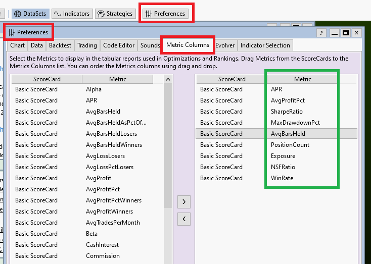
In this window you can choose all the Performance metrics you find important for optimization. A good set is mentioned in Post #18.
Why does this window even exist?
Well, we talk about execution performance here. If all extensions are installed WL knows about several hundred (!) performance metrics (I counted more than 500 the last time). While the calculation of a single metric may be fast, the calculation of all available metrics can take a considerable and quite noticeable amount of time.
We want our (hundreds of) optimization iterations to run as fast as possible and one way to achieve this is by limiting the number of performance metrics calculated after each backtest executed by the optimizer.
This forces you to think about the results you want to see before optimization is started.
As a good start, if you make the window look like the screenshot above we are ready to go!
Preferences->Metric Columns
In this window you can choose all the Performance metrics you find important for optimization. A good set is mentioned in Post #18.
Why does this window even exist?
Well, we talk about execution performance here. If all extensions are installed WL knows about several hundred (!) performance metrics (I counted more than 500 the last time). While the calculation of a single metric may be fast, the calculation of all available metrics can take a considerable and quite noticeable amount of time.
We want our (hundreds of) optimization iterations to run as fast as possible and one way to achieve this is by limiting the number of performance metrics calculated after each backtest executed by the optimizer.
This forces you to think about the results you want to see before optimization is started.
As a good start, if you make the window look like the screenshot above we are ready to go!
New to this topic, optimization is even broader than I think. Thank you Dr. Koch for the work!
I also hope you will talk about how to interpret different tables like surface graph and financial tables.Optimize and scoreCard.
Also a detailed tutorial on the financieric.NPL extension would be great.
In Post #23 you said “unseen data”, what does that mean? Monte Carlo ?
I have seen several times on posts that for optimization we do not use a “peek” indicator. What are these indicators (I speak French and I have difficulty translating).
In Post #30 you said "Position size: I always use equity percentage", why not otherwise?
the problem I think with equity percentage is its compound return side, so a exponential graph. I am insinuating that the first positions will be the most important over time, so a bad start would change everything (especially in intraday optimization, in investment I see the interest). I would tend to use "pos max Risk %" which will take the same position size over time, but you have to use a thousand billion capital + margin to not have NSF.
What do you think?
Otherwise, I'm interested in the Advanced Pos Sizer, is there one that can be optimized? or is it better to start with the equity percentage and then change? (as you said after the exploration)
QUOTE:
how to interpret different tables like surface graph and financial tables.Optimize and scoreCard
I'll discuss these later.
I consider the following questions off-topic. Please start another discussion thread for these:
* tutorial on the finantic.NLP extension
* I have seen several times on posts that for optimization we do not use a “peek” indicator. What are these indicators (I speak French and I have difficulty translating).
* In Post #30 you said "Position size: I always use equity percentage", why not otherwise?
the problem I think with equity percentage is its compound return side, so a exponential graph.
I am insinuating that the first positions will be the most important over time,
so a bad start would change everything (especially in intraday optimization, in investment I see the interest).
I would tend to use "pos max Risk %" which will take the same position size over time, but you have to use a thousand billion capital + margin to not have NSF.
* I'm interested in the Advanced Pos Sizer, is there one that can be optimized?
or is it better to start with the equity percentage and then change?
QUOTE:
In Post #23 you said “unseen data”, what does that mean?
Whenever you run a backtest (and it does not matter if it is a single, manually started backtest or a set of backtests started by the optimizer), whenever you run a backtest and use the results to change your strategy, then you adapt your startegy with all its logic, parameters and settings to the data used in the backtest. In fact it is always a small step direction curve-fitting/over-optimization. After many (and often not so many) such steps you end up with a strategy that works great on your backtest data - and will fail for any other data, i.e. in the future.
One counter-measure is called "Cross-Validation": Run your strategy on data that was not used during the backtest. Some call it "unseen data" because the strategy had never seen/used/worked on this data. We'll talk about "Cross-Validation" and its importance later.
With all settings in place we are now ready to go:
Step 2: Start Optimization
Open your Strategy and click the Optimize Button (see red rectangle #1). This will add the Optimization tab (see green rectangle):
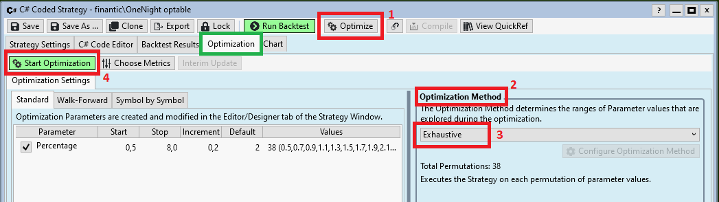
Being in Exploration Mode and using the OneNight strategy with one optimizable parameter (see above)
we choose the Optimization method "Exhaustive" (see red rectangles #2 and #3.
Now it is time to click "Start Optimization (see red rectangle #4).
This will run a few seconds:

After optimization has finished a few more tabs are added to the Optimization tab of our strategy window. Now we are ready for the next step.
Step 2: Start Optimization
Open your Strategy and click the Optimize Button (see red rectangle #1). This will add the Optimization tab (see green rectangle):
Being in Exploration Mode and using the OneNight strategy with one optimizable parameter (see above)
we choose the Optimization method "Exhaustive" (see red rectangles #2 and #3.
Now it is time to click "Start Optimization (see red rectangle #4).
This will run a few seconds:
After optimization has finished a few more tabs are added to the Optimization tab of our strategy window. Now we are ready for the next step.
Step 3: Inspecting Optimization Results
We start with looking at he Tabular tab that contains a table with all available results form the optimization run:
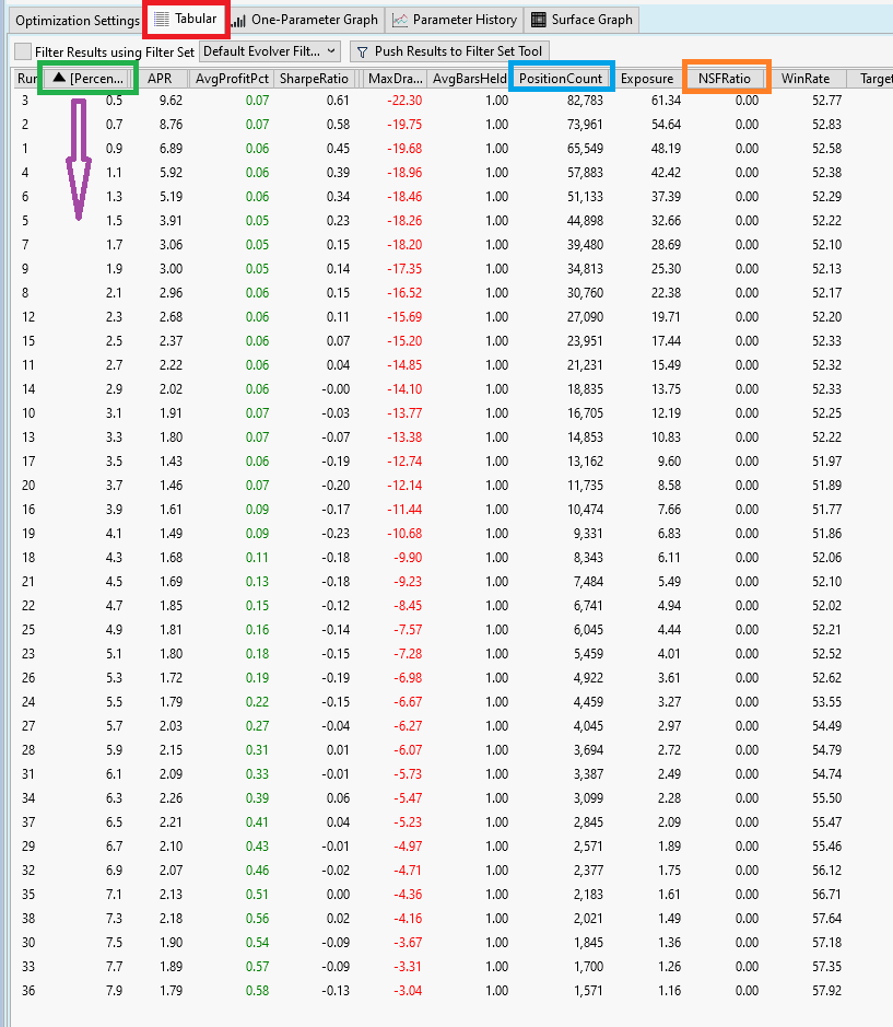
This table has three parts:
1. run number. Not very important
2. All optimizable parameters (here we have just one: Percentage)
3. Performance Metrics. These are all the metrics we chose in Preferences->Metric Columns (see Post #31)
First we quickly inspect the 10. column named NSFRatio (see orange rectangle). We check that indeed all runs have a NSF ratio of 0.0. This was one goal during Exploration Mode. (see Post #30, Position Sizing)
The second column, named "Percentage" (see red rectangle) contains our optimizable parameter. I sorted this column ascending (see violet arrow) to make all other results more understandable.
From Column 2 "Percentage" we see that the optimizer did exactly what we instructed it to do: It run a backtest for each parameter value between 0.5 and 7.9 with an increment of 0.1.
As an example we can look at the 8th column, named "PositionCount" and see how the parameter Percentage influences the number of open positions.
All the information is there, but it is hard to read raw values form a table. Thus lets proceed with the next step.
We start with looking at he Tabular tab that contains a table with all available results form the optimization run:
This table has three parts:
1. run number. Not very important
2. All optimizable parameters (here we have just one: Percentage)
3. Performance Metrics. These are all the metrics we chose in Preferences->Metric Columns (see Post #31)
First we quickly inspect the 10. column named NSFRatio (see orange rectangle). We check that indeed all runs have a NSF ratio of 0.0. This was one goal during Exploration Mode. (see Post #30, Position Sizing)
The second column, named "Percentage" (see red rectangle) contains our optimizable parameter. I sorted this column ascending (see violet arrow) to make all other results more understandable.
From Column 2 "Percentage" we see that the optimizer did exactly what we instructed it to do: It run a backtest for each parameter value between 0.5 and 7.9 with an increment of 0.1.
As an example we can look at the 8th column, named "PositionCount" and see how the parameter Percentage influences the number of open positions.
All the information is there, but it is hard to read raw values form a table. Thus lets proceed with the next step.
Step 4: One-Parameter Graph: Number of Positions
We have seen it already in the Tabular result from the previous post: There is an interesting relation between parameter "Percentage" and number of positions ("PositionCount"). We can visualize this relationship in the tab "One-Parameter-Graph":
We selected "PositionCount" for "Graph metric". Here is the result:
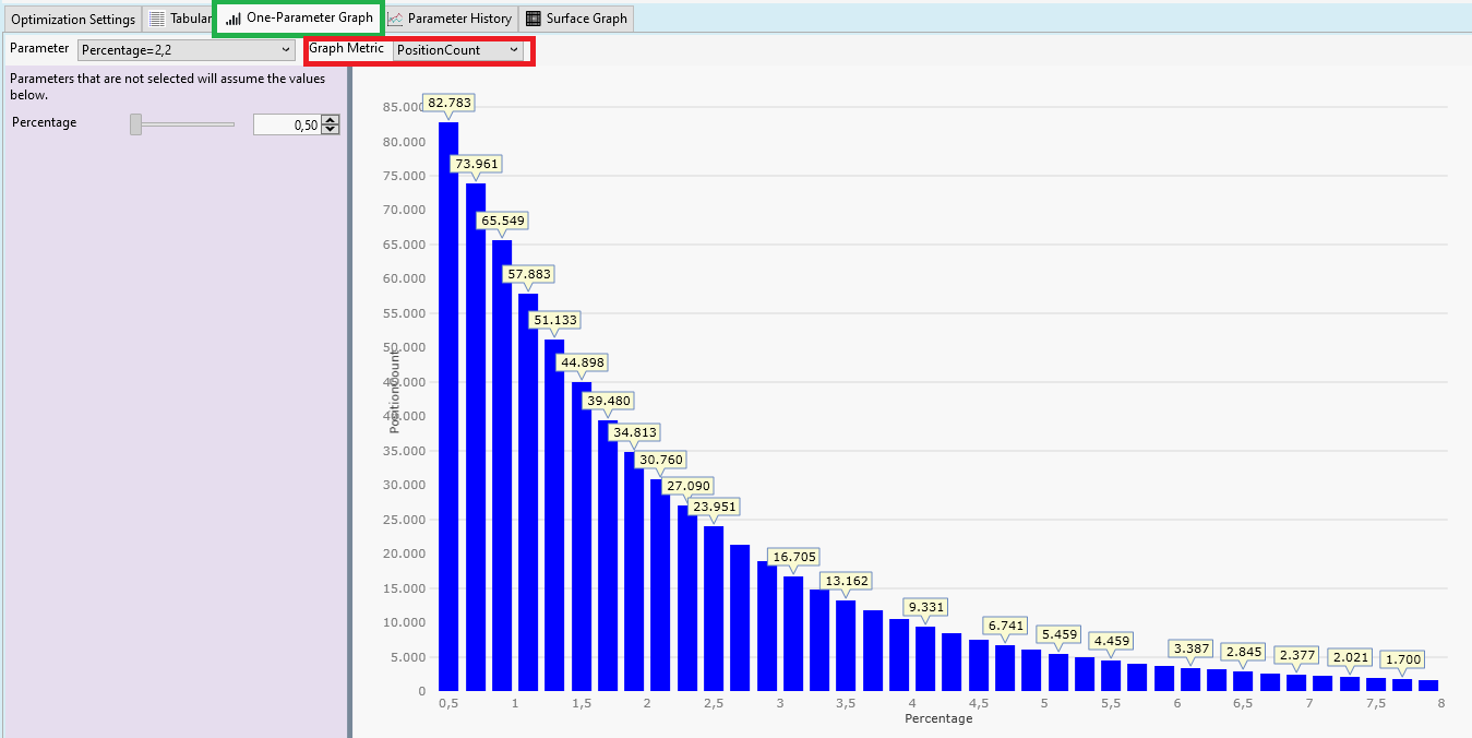
Our optimizable parameter "Percentage" is shown on the X-Axis. The number of positions is shown on the Y-Axis. We see a very clear relationship: The smaller "Percentage", the more positions.
This was expected. "Percentage" is the distance prices have to travel between yesterday's close price and the limit price before a position is entered.
The larger this distance, the less likely the limit price will be reached. This is a very basic property of random walks (and a price series is mostly a random walk).
You'll see a very similar picture for all long limit entry strategies. This is one of the clearest, most robust results you'll ever see when inspecting optimization results.
We have seen it already in the Tabular result from the previous post: There is an interesting relation between parameter "Percentage" and number of positions ("PositionCount"). We can visualize this relationship in the tab "One-Parameter-Graph":
We selected "PositionCount" for "Graph metric". Here is the result:
Our optimizable parameter "Percentage" is shown on the X-Axis. The number of positions is shown on the Y-Axis. We see a very clear relationship: The smaller "Percentage", the more positions.
This was expected. "Percentage" is the distance prices have to travel between yesterday's close price and the limit price before a position is entered.
The larger this distance, the less likely the limit price will be reached. This is a very basic property of random walks (and a price series is mostly a random walk).
You'll see a very similar picture for all long limit entry strategies. This is one of the clearest, most robust results you'll ever see when inspecting optimization results.
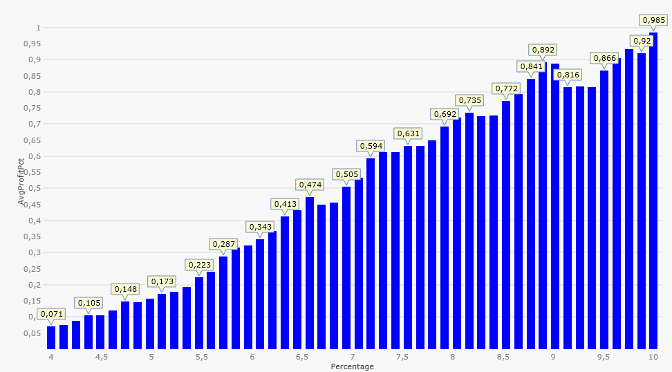
Step 5: One-Parameter Graph: Average Profit per Trade in Percent
Now we choose the Graph Metric "AvgProfitPct" which results in this picture:
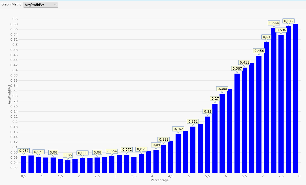
This time we see the average profit per trade in percent on the Y-Axis.
For me "Average Profit per Trade" is the most important metric during exploration mode because it is a very direct measurement of the merit of the trading logic.
Back to the picture:
The profit gets bigger if "Percentage" is chosen to be 4% or more.
This is not expected and a clear violation of the random walk hypothesis!
Random walk theory says that it does not matter where we start with our price movements. Up and down have the same probability.
Our result says: If we start 4 or more percent below yesterday's close, an up-movement (profit) has a higher probability than a down-movement (loss).
This is called an edge. An advantage compared to random price movements.
This is something you don't see all too often when searching for a profitable trading logic.
We also note: It happens for limit orders more than 4% below yesterday's close only.
Now we choose the Graph Metric "AvgProfitPct" which results in this picture:
This time we see the average profit per trade in percent on the Y-Axis.
For me "Average Profit per Trade" is the most important metric during exploration mode because it is a very direct measurement of the merit of the trading logic.
Back to the picture:
The profit gets bigger if "Percentage" is chosen to be 4% or more.
This is not expected and a clear violation of the random walk hypothesis!
Random walk theory says that it does not matter where we start with our price movements. Up and down have the same probability.
Our result says: If we start 4 or more percent below yesterday's close, an up-movement (profit) has a higher probability than a down-movement (loss).
This is called an edge. An advantage compared to random price movements.
This is something you don't see all too often when searching for a profitable trading logic.
We also note: It happens for limit orders more than 4% below yesterday's close only.
There are many ways to proceed from here. To make most out of this tutorial we choose the following path:
Inspired from the results in the previous post we decide to concentrate on the parameter region from 4.0 percent upwards. Here we expect quite large values for Average Profit per Trade.
-> We change the start value of parameter "Percentage" to 4.0
-> We also change the stop value to 10.0 because the plots in Posts #37 (PositionCount) and Post #38 (AvgProfitPct) look like there is some more interesting data to the right (i.e. for larger Percentage values)
We also change our Optimization Method to "Grid Search" because I am too lazy to calculate the necessary Increment values for our parameter. Instead I use the settings of "Grid Search" to specify the requested number of iterations directly (see also Post #15):
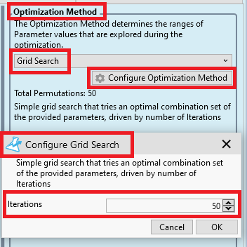
We chose 50 Iterations because this gives us a good resolution in the plots and does not take too much time to calculate.
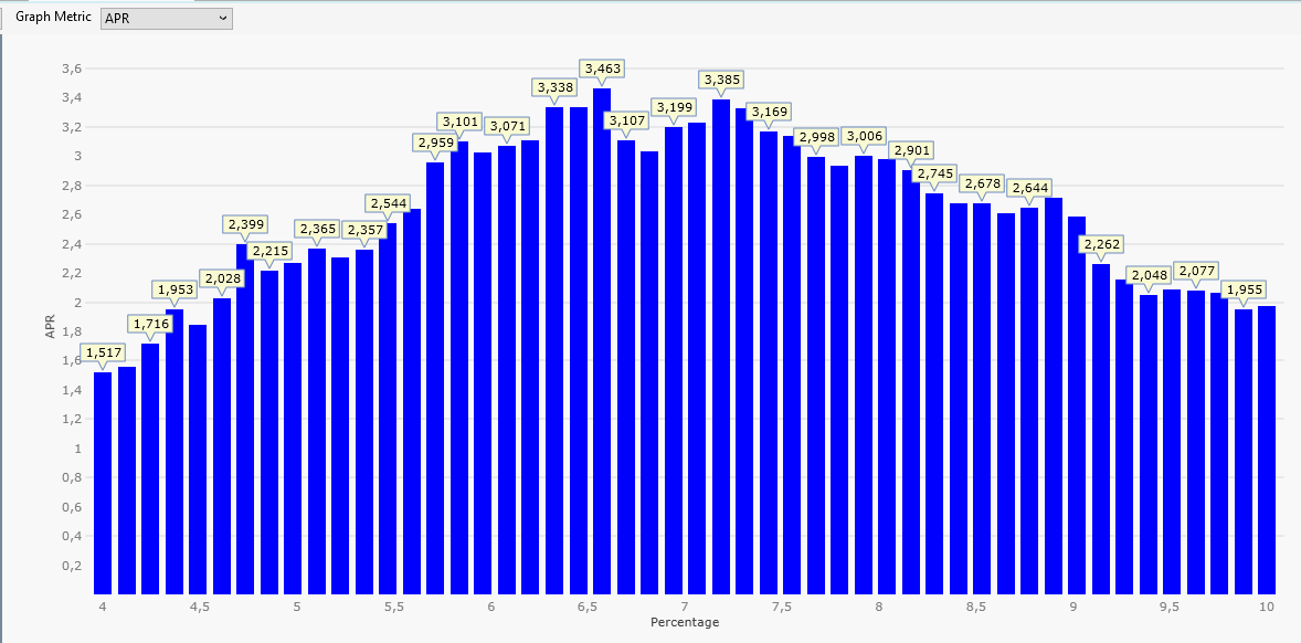
With all these changes in place we produce the "AvgProfitPct vs. Percentage" plot again:
We note that the X-Axis now shows parameter values between 4.0 and 10.0 (as planned) and the resolution (number of data points) is somewhat better than before. We also note that the general tendency in the data continues for Percentage values larger than 8% - interesting.
Inspired from the results in the previous post we decide to concentrate on the parameter region from 4.0 percent upwards. Here we expect quite large values for Average Profit per Trade.
-> We change the start value of parameter "Percentage" to 4.0
-> We also change the stop value to 10.0 because the plots in Posts #37 (PositionCount) and Post #38 (AvgProfitPct) look like there is some more interesting data to the right (i.e. for larger Percentage values)
We also change our Optimization Method to "Grid Search" because I am too lazy to calculate the necessary Increment values for our parameter. Instead I use the settings of "Grid Search" to specify the requested number of iterations directly (see also Post #15):
We chose 50 Iterations because this gives us a good resolution in the plots and does not take too much time to calculate.
With all these changes in place we produce the "AvgProfitPct vs. Percentage" plot again:
We note that the X-Axis now shows parameter values between 4.0 and 10.0 (as planned) and the resolution (number of data points) is somewhat better than before. We also note that the general tendency in the data continues for Percentage values larger than 8% - interesting.
Step 6: One-Parameter Graph: APR
After all we are only mildly interested in PositionCount or AvgProfitPct. What really counts is the overall profit of our trading strategy.
We switch Graph Metric to APR:
PositonCount became smaller for larger Percentages.
AvgProfitPct became larger for larger Percentages.
APR is the product of both (times some scaling) and has a clear maximum of 3,5% for a Percentage setting of 6.6.
This is a clear and simple result - or is it?
Before you start realtime trading of the OneNight strategy with a Percentage setting of 6.6% lets do some more experiments:
The plot above was created with a year range from 2020 to 2022 (three years).
If we change the year range slightly (form 2019 to 2021, three years) we get this plot:
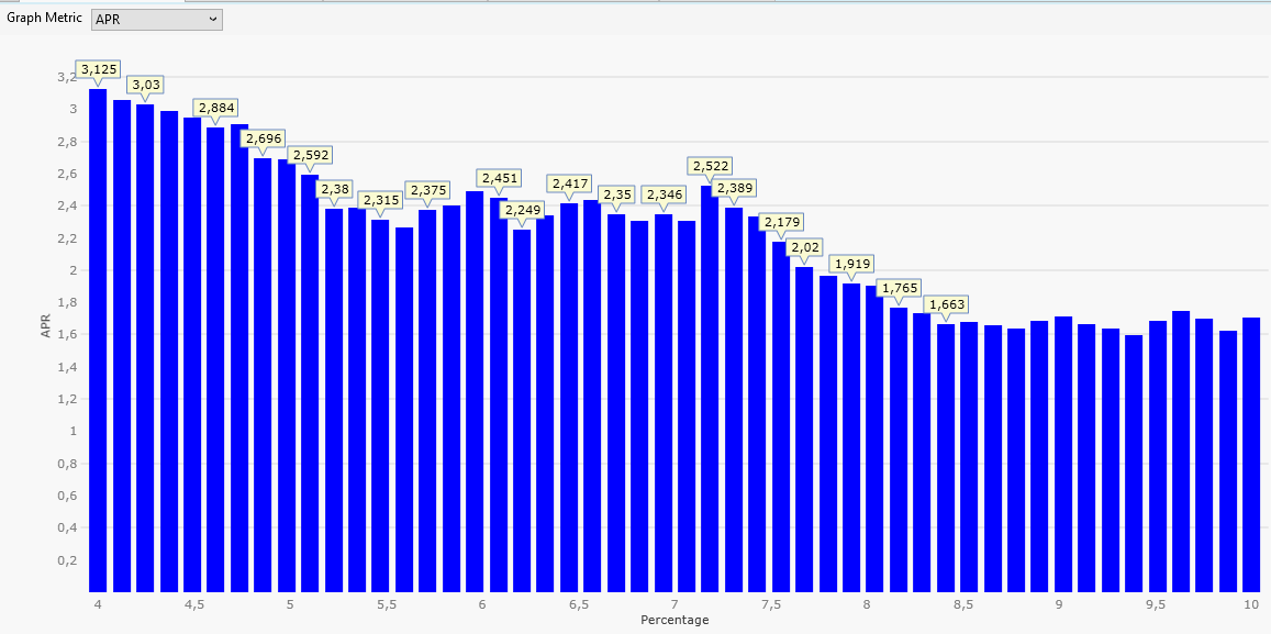
A tiny change in our backtest data (we shifted a three-year interval by one year) caused a massive change in the APR results.
This means: Optimization results are volatile. They may change a lot if (for example) the data range is changed.
THIS IS IMPORTANT!
Never rely on a single optimization result.
Never dream about a clearly visible maximum like in the first plot of this Post. Such a maximum will go away if you shift (even so slightly) into the future.
Conclusion: We have to make much more effort to get usable (and tradable) results. A single optimization run is too fragile, volatile, misleading, and so forth.
After all we are only mildly interested in PositionCount or AvgProfitPct. What really counts is the overall profit of our trading strategy.
We switch Graph Metric to APR:
PositonCount became smaller for larger Percentages.
AvgProfitPct became larger for larger Percentages.
APR is the product of both (times some scaling) and has a clear maximum of 3,5% for a Percentage setting of 6.6.
This is a clear and simple result - or is it?
Before you start realtime trading of the OneNight strategy with a Percentage setting of 6.6% lets do some more experiments:
The plot above was created with a year range from 2020 to 2022 (three years).
If we change the year range slightly (form 2019 to 2021, three years) we get this plot:
A tiny change in our backtest data (we shifted a three-year interval by one year) caused a massive change in the APR results.
This means: Optimization results are volatile. They may change a lot if (for example) the data range is changed.
THIS IS IMPORTANT!
Never rely on a single optimization result.
Never dream about a clearly visible maximum like in the first plot of this Post. Such a maximum will go away if you shift (even so slightly) into the future.
Conclusion: We have to make much more effort to get usable (and tradable) results. A single optimization run is too fragile, volatile, misleading, and so forth.
This series could shape up into an actual publishable book.
I already called dibs on the blog!
In Post #40 we have seen that it is very important to check optimization results from one data range against results from another data range. This idea is called "Cross Validation" (see https://en.wikipedia.org/wiki/Cross-validation_(statistics)).
In its simplest form it uses two intervals (like above, in Post #40).
Of course it is possible to always run two optimizations with different data range settings but this process is cumbersome and error-prone and involves quite some copy-paste-to-excel magic to compare results side-by-side.
It is much better to let some software help and assist us.
Within Wealth-Lab an automatic two-interval cross-validation method is implemented in a somewhat unexpected way: It is done by the Insample/Out of Sample Scorecard (or IS/OS for short) (part of the finantic.ScoreCards extension).
The name comes from the names given to the two intervals in such a Cross-Validation. One interval is called "Insample" and usually used to learn, train or otherwise adapt parameters. The second interval is called "Out-of-Sample" and usually used to check results. (In the examples above there is no "learning", we stick to these names nonetheless.)
Let's put the IS/OS ScoreCard to work!
Cross Validation with the Insample/Out of Sample Scorecard
The IS/OS Scorecard works by splitting the available data (the data range of our backtest) into two intervals called "Insample (IS) and "Out-of-Sample" (OS).
This is specified in Preferences->Intervals:
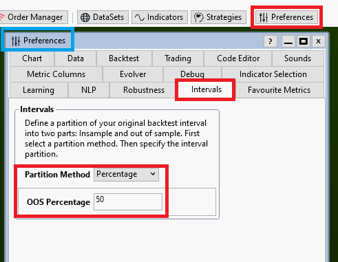
For now we choose the Partition Method "Percentage" and an OOS Percentage of 50%.
This will divide our original data range into two equally sized parts.
Next we go to Preferences->Metric Columns.
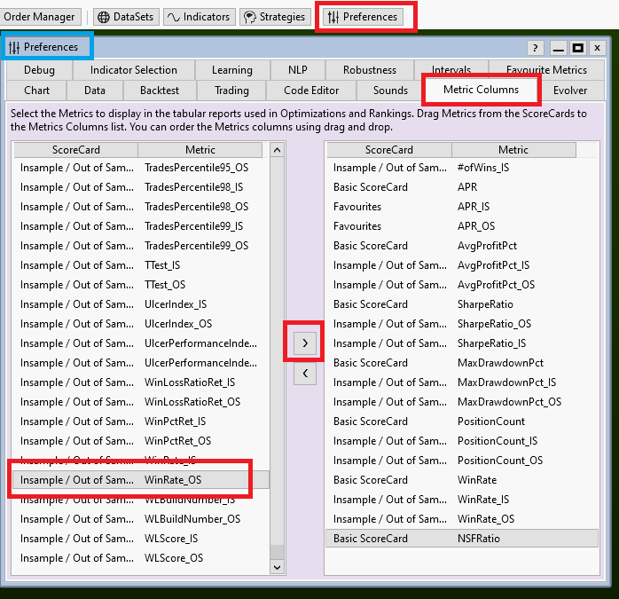
The left pane contains an IS version and an OS version of each available performance metric (provided by the Insample/Out of Sample ScoreCard).
For example there is APR form Basic ScoreCard and also APR_IS and APR_OS from the IS/OS ScoreCard.
For each Metric in the right pane we add the IS version and the OS version to make it look like in the screenshot above.
For every (interesting or important) performance metric there are now three versions like APR, APR_IS and APR_OS.
(We have NSFRatio just once. If this is 0.0 we are happy)
(There is one additional dummy metric "#ofWins_IS" at the top. this avoids an unexplainable bug, please do this the same way and: don't ask)
The IS/OS Scorecard works by splitting the available data (the data range of our backtest) into two intervals called "Insample (IS) and "Out-of-Sample" (OS).
This is specified in Preferences->Intervals:
For now we choose the Partition Method "Percentage" and an OOS Percentage of 50%.
This will divide our original data range into two equally sized parts.
Next we go to Preferences->Metric Columns.
The left pane contains an IS version and an OS version of each available performance metric (provided by the Insample/Out of Sample ScoreCard).
For example there is APR form Basic ScoreCard and also APR_IS and APR_OS from the IS/OS ScoreCard.
For each Metric in the right pane we add the IS version and the OS version to make it look like in the screenshot above.
For every (interesting or important) performance metric there are now three versions like APR, APR_IS and APR_OS.
(We have NSFRatio just once. If this is 0.0 we are happy)
(There is one additional dummy metric "#ofWins_IS" at the top. this avoids an unexplainable bug, please do this the same way and: don't ask)
With all these preparations in place we can run an optimization again, this time we choose Strategy Settings->Data Range From 2013 to 2022 (10 years).
Tabular results now looks like this:
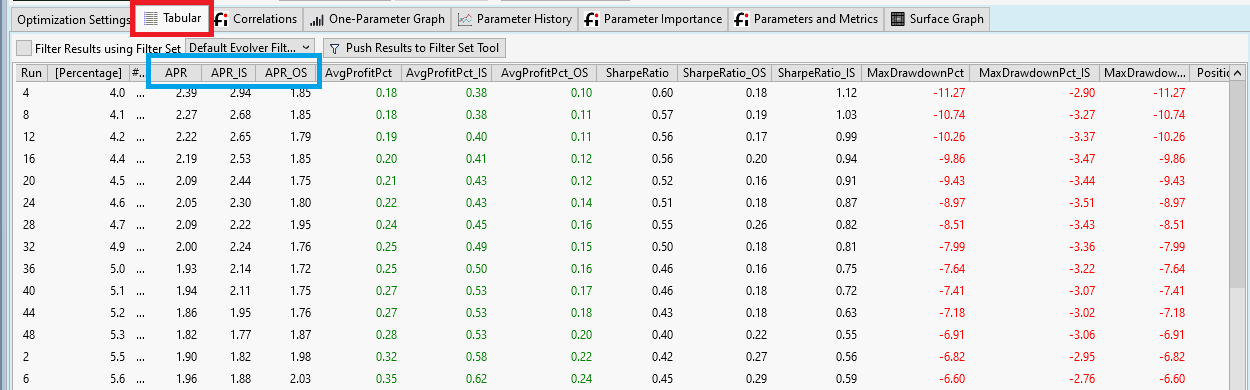
Instead of a single column for "APR" (like in the runs before, see Post #35) we now have three columns: APR, APR_IS and APR_OS. And similar for all other performance metrics.
What happened can be understood as three optimization runs at the same time:
1. the original data range 2013 to 2022, producing the APR result.
2. An Insample run (2013 to 2017) producing the APR_IS result.
3. An Out-of-Sample run (2018 to 2022) producing the APR_OS result.
Lets pause for a moment and let this sink in...
Tabular results now looks like this:
Instead of a single column for "APR" (like in the runs before, see Post #35) we now have three columns: APR, APR_IS and APR_OS. And similar for all other performance metrics.
What happened can be understood as three optimization runs at the same time:
1. the original data range 2013 to 2022, producing the APR result.
2. An Insample run (2013 to 2017) producing the APR_IS result.
3. An Out-of-Sample run (2018 to 2022) producing the APR_OS result.
Lets pause for a moment and let this sink in...
I really don't like to read through hundreds of table values, and the One-Parameter Graph can show just two columns (one metric vs. one parameter) at a time so time has come for another optimization results viewer:
The Parameters and Metrics Optimization Results Visualizer
This visualizer (part of the finantic.Optimizer extension) is designed to show up to two parameters and up to two performance metrics at the same time and allows for some very interesting plots.
For now we use it to show the same results as in Post #37 (PositionCount), but this time for two intervals (IS/OS).
In Strategy Window->Optimization open the "Parameters and Metrics" tab:
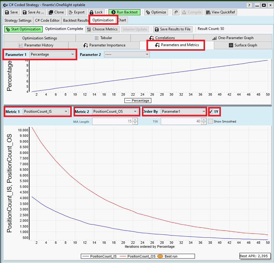
The upper panel is the parameter panel. We have just one parameter "Percentage" so we choose this one for "Parameter1" and leave "Parameter2" empty.
The lower panel is for performance metrics. we choose:
Metric 1: PositionCount_IS: The number of positions in the IS interval
Metric2: PositionCount_OS: The number of positions in the OS interval
Order By: Parameter 1: We want to produce a plot similar to the one in Post #37, we want the parameter values to increase from left to right.
Please click the "1Y" checkbox which will make both curves use the same Y-Axis.
This visualizer works a bit different from the "One-Parameter Graph". It uses an abstract "Iteration Number" for the X-Axis. (The reason for this will later become clear).
Both panels, parameters and metrics use the same X-Axis. If you want to know the parameter value for Iteration#20 you need to look it up in the upper (parameter) panel. Here you'll find a parameter value of about 6.3 for Iteration#20.
In the plot above we see PositionCount for both the IS interval (blue line) and the OS interval (red line). As discussed above there is a clear relationship between parameter values ("Percentage", the distance between yesterday's close price and our limit entry price) and the number of positions. This relationship holds nicely for both, the IS and the OS interval.
The Parameters and Metrics Optimization Results Visualizer
This visualizer (part of the finantic.Optimizer extension) is designed to show up to two parameters and up to two performance metrics at the same time and allows for some very interesting plots.
For now we use it to show the same results as in Post #37 (PositionCount), but this time for two intervals (IS/OS).
In Strategy Window->Optimization open the "Parameters and Metrics" tab:
The upper panel is the parameter panel. We have just one parameter "Percentage" so we choose this one for "Parameter1" and leave "Parameter2" empty.
The lower panel is for performance metrics. we choose:
Metric 1: PositionCount_IS: The number of positions in the IS interval
Metric2: PositionCount_OS: The number of positions in the OS interval
Order By: Parameter 1: We want to produce a plot similar to the one in Post #37, we want the parameter values to increase from left to right.
Please click the "1Y" checkbox which will make both curves use the same Y-Axis.
This visualizer works a bit different from the "One-Parameter Graph". It uses an abstract "Iteration Number" for the X-Axis. (The reason for this will later become clear).
Both panels, parameters and metrics use the same X-Axis. If you want to know the parameter value for Iteration#20 you need to look it up in the upper (parameter) panel. Here you'll find a parameter value of about 6.3 for Iteration#20.
In the plot above we see PositionCount for both the IS interval (blue line) and the OS interval (red line). As discussed above there is a clear relationship between parameter values ("Percentage", the distance between yesterday's close price and our limit entry price) and the number of positions. This relationship holds nicely for both, the IS and the OS interval.
Next we are going to create the IS/OS version of the AvgeProfitPct plot shown in Post #39.
We choose:
Metric 1: AvgProfitPct_IS
Metric 2: AvgProfitPct_OS
We leave Order By: Parameter1 and the checked 1Y untouched.
Here is the result:
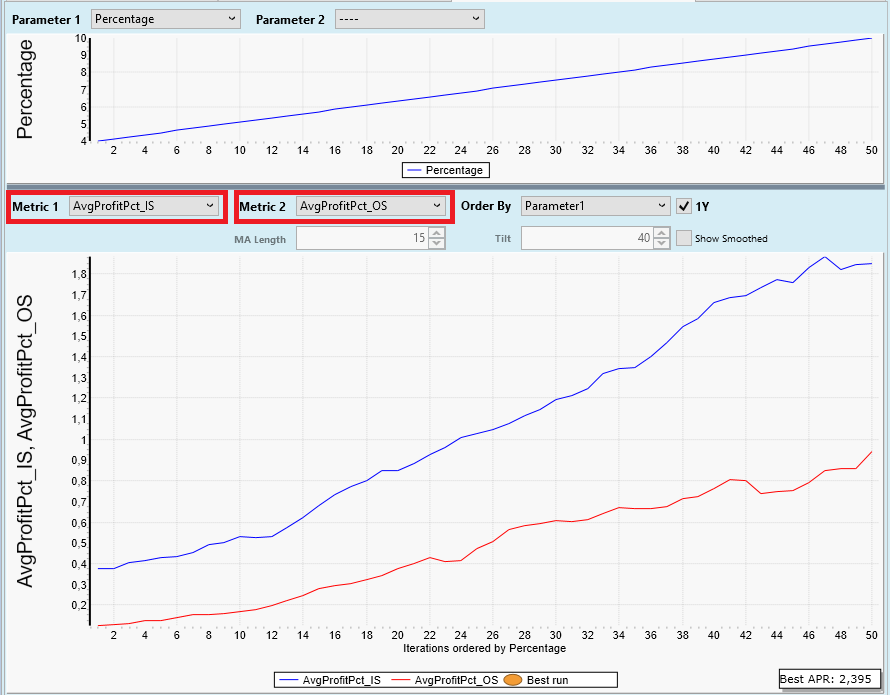
We notice that the nice (and unexpected) relationship between "Percentage" and "AvgProfitPct" that we found in Post #39 also holds nicely for both the IS and OS intervals.
So the basic "edge" of our trading system seems to be a stable one.
Discoveries
If we look closer, we notice that in one interval (OS, red) there are more trades (and lower AvgProfit) and in the other (IS, blue) less trades and higher AvgProfit.
This may be a hint that the overall volatility of the market changes with time (making our limit at x% more probable) and that the AvgProfit in fact does not depend on a percentage but on volatility. Lets keep this in mind for later investigation.
Allow me another remark: It is possible to see these things without the IS/OS Scorecard and with the One-Parameter Graph only. It is just much harder and more time-consuming to see these results (and you need to know what you are looking for).
We choose:
Metric 1: AvgProfitPct_IS
Metric 2: AvgProfitPct_OS
We leave Order By: Parameter1 and the checked 1Y untouched.
Here is the result:
We notice that the nice (and unexpected) relationship between "Percentage" and "AvgProfitPct" that we found in Post #39 also holds nicely for both the IS and OS intervals.
So the basic "edge" of our trading system seems to be a stable one.
Discoveries
If we look closer, we notice that in one interval (OS, red) there are more trades (and lower AvgProfit) and in the other (IS, blue) less trades and higher AvgProfit.
This may be a hint that the overall volatility of the market changes with time (making our limit at x% more probable) and that the AvgProfit in fact does not depend on a percentage but on volatility. Lets keep this in mind for later investigation.
Allow me another remark: It is possible to see these things without the IS/OS Scorecard and with the One-Parameter Graph only. It is just much harder and more time-consuming to see these results (and you need to know what you are looking for).
To complete this string of thoughts we are going to produce an IS/OS version of the plots shown in Post #40 (APR vs. Percentage), same information plotted in one graph instead of two:
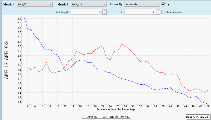
What is this? We have seen nice and stable relationships for PositionCount and AvgProfitPct. But the APR graph looks chaotic?
We remember: APR := PositionCount * AvgPrPct * scaling
PositionCount goes down with higher parameter=Percentage settings
AvgPrPct goes up with higher parameter=Perceantage settings.
So the product of both is supposed to be (more or less) constant(!)
And let me tell you what I see in the APR_IS/APR_OS plot above:
I see a constant APR of about 2.0%, for parameter=Percentage values between 5% and 8% (Iteration Numbers 10 to 35)
For me, the rest are statistical fluctuations around this APR value of 2.0%.
This means: It does not matter too much which parameter=Percentage value we choose when it comes to the resulting APR value.
This may come as a surprise. But if you look at optimizer results you should always squint your eyes and imagine a (rather broad) band of noise around the data you see.
QUOTE:
APR of about 2.0%
I hear you saying "Who cares about 2%?"
So let me clarify:
We are still in Exploration Mode. In order to get zero NSF positions (and thereby minimize analysis noise and some other unwanted effects) we chose a small position size of 1%. This resulted in an APR of 2%. When we add more "realism" at a later stage we'll use a position size closer to 10% which should result in an APR of 20%. I hope this sounds better in your ears.
Thank you, DrKoch. Really great article especially when red by a person new to Wealth-Lab.
It would be very interesting to see continuation of this article. When SMAC optimization method comes into play?
It would be very interesting to see continuation of this article. When SMAC optimization method comes into play?
I got distracted by the update wave caused by Build77.
After that I plan to continue here.
I guess this Optimizer Tutorial is currently 30% complete.
After that I plan to continue here.
I guess this Optimizer Tutorial is currently 30% complete.
Your Response
Post
Edit Post
Login is required